Control blocks
Control blocks are those related to the creation of control loops.
PID
PID Static block allows the user to build a PID (Proportional, Integral and Derivative) controller with fixed gains.

PID block
As can be seen in the figure above, PID Static block has 2 ![]() buttons that enable or disable the block to be commanded from the 1x PDI Tuning software.
buttons that enable or disable the block to be commanded from the 1x PDI Tuning software.

PID block - Command buttons
The first button is for activating ‘Command PID’ and the second one is for the ‘Autotune’ command. For more information on these commands, please refer to the Tuning section of the 1x PDI Tuning user manual.
Each command button has a different ID that allows the user to identify it during the command.
Note
To avoid disabling a block by mistake, the following warning message appears when disabling it:
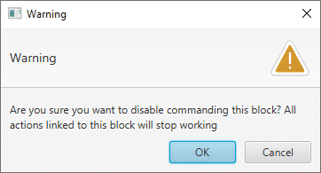
Warning message when disabling the command
The PID mathematical implementation in Veronte Autopilot 1x is the following:
\[C = Kp + \frac{1}{T_i} \cdot I F(z) + \frac{Td}{\tau + DF(z)}\]Where:
\[DF(z) = T_s \cdot \frac{z}{z-1} \quad ; \quad IF(z) = \frac{T_s}{2} \cdot \frac{z+1}{z-1} \quad ; \quad LPF(s) = \frac{1}{\tau s +1}\]Inputs
 yc: Target value, desired set-point of the controlled variable. y: Closed loop, value of the controlled variable. (Optional) dy: Derivative of the controlled variable (computed numerically from ‘y’ if not connected). (Optional) usat: Previously applied control action after saturation (used for anti-windup and respect). If not connected a value of zero is assumed. (Optional) ff: Feed-forward control, this value is added to the ‘u’ output before applying the output limits. If not connected a value of zero is assumed.
 (Optional) respect: When TRUE the output ‘u’ is equal to the input ‘usat’ and the integral component is estimated with the information in ‘y’ and ‘yc’. When FALSE the PID works as usual. If not connected a value of FALSE is assumed. (Optional) enable integral: When TRUE the the PID works as usual. When FALSE the integral is exponentially discharged. If not connected a value of TRUE is assumed.
Outputs
u: Control output after applying PID limits. p: Proportional part of the output before the PID limits are applied. i: Integral part of the output before the PID limits are applied. d: Derivative part of the output before the PID limits are applied.Configuration menu:
Double click on the block to open its configuration menu.
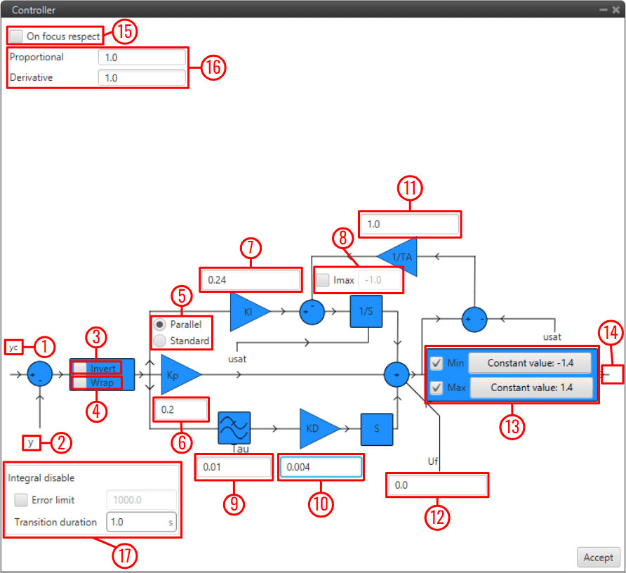
PID block configuration
yc: Input variable.
y: Feedback variable.
Invert: Apply a -1 gain .
Wrap: Perform a [-pi, pi] wrap.
Parallel/Standard: In parallel mode, PID gains are independent. In standard mode, I & D gains are scaled by P gain.
KP: Proportional gain.
1/TI: Integral gain.
Imax: Maximum value for integral term. Value must be possitive and the limit applied is symmetrical ([-Imax, Imax]).
tau: Time constant for the derivative term first order LPF.
TD: Derivative gain.
TA: Anti-windup gain. Recommended value around x10 KI. Unloads integral term if output is saturated.
Uf: Output offset. Feedforward value is also applied at this point.
Min/Max: Output limits. Users can manually enter a value or select a variable.
u: PID output.
On focus respect: If respect is enabled, when the PID is first executed, an initial I value will be applied so that ‘u’ = ‘usat’ for the first iteration.
Proportional/Derivative Beta: yc scaling for proportional and derivative terms. Unless necessary, value should always be 1.
Integral disable: Disables integral term if (yc - y) > Error limit.
Tip
Remember to always use ‘wrap’ for direction controllers, such as ‘Heading’ or ‘Yaw’ PIDs. This will allow the UAV to always turn in the right direction.
T-Sched PID
TSched PDI block is a PID (Proportional, Integral and Derivative) controller with table scheduled parameters. It allows to scale most PID parameters using an external variable, usually the speed (Ground speed or IAS).

TSched PID block
It works in a very similar way to the PID Static block, except that in that block the gains are fixed and in the TSched block they are adjusted for different values of the input variable.
For this reason, the inputs and outputs are the same, but in this block an additional input is added:
Input
var: Scaling variable for gain scheduling used to interpolate in the table to obtain the PID parameters.Configuration menu
Double click on the block to open its configuration menu.

TSched PID block configuration
In this block, the PID gains for the different values of the input variable must be entered in the table above instead of in the diagram. To add more values, simply click on
 and to remove them, click on
  .
.If the variable is outside the limits, the values of the closest point will be applied. Values between points are linearly interpolated.
In addition, clicking on “Table Generator” will bring up another configuration menu:
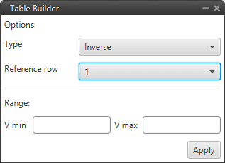
TSched PID block configuration - Table Generator
This is another option to enter the PID gains for different values of the input variable, instead of manually entering all the gains, the Table Generator will generate them according to the parameters to be configured:
Type: Depending on the type of function selected, the gains are calculated differently.
Inverse: It will calculate the different gains with an inverse function.
Proportional: It will calculate the different gains with a proportional function.
Quadratic: It will calculate the different gains with a quadratic function.
Type
Result (\(K_p\))
Inverse
\(K_{p_i} \frac{V}{V_i}\)
Proportional
\(K_{p_i} \frac{V_i}{V}\)
Quadratic
\(K_{p_i} \frac{V_i^2}{V^2}\)
Reference cow: Users must select the reference values from which the other values will be calculated.
Range: The minimum and maximum values of the input variable between which the gains have to be calculated have to be defined.
Then just click on “Apply” and the maximum number of points that the table allows will be generated.
Example
Example of Table Generator
ECU Control
The ECU Control block allows to control the winding speed of the microjets and to ensure safe motor operation based on PID control and shaft speed for the microjets.
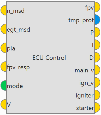
ECU Control block
The ECU Control mathematical algorithm is based on a PID scheduler, this PID control has been used because the dynamics of the motor changes with RPM so it is very different at low and high speed. For more information on PID Scheduler control, see T-Sched PID section of this manual.
First, the PLA magnitude is converted in commanded speed based in a look-up table. This information must be provided by engine producer.
To protect from a common problem of engines the commanded speed is limited. For this, first, the maximum speed is limited to the configurable parameter \(N_{max}\) to ensure mechanical integrity.
Then, engine acceleration is limited to protect from compressor surge, so the maximum speed rate is limited to a configurable parameter in block, \(\dot{N}_{max}\).
Finally, engine deceleration is limited to protect from blow out, so the minimum speed rate is limited to a configurable parameter in block, \(\dot{N}_{min}\).
If EGT is less than the maximum value (configurable), the error magnitude in speed is minimized with a PID scheduler: \(e = y - yc = N - N (PLA)\).
And the control output of this block is the FPV commanded to engine.
If EGT measurement is higher than maximum temperature (configurable \(EGT_{max}\)), a protection protocol is initiated and the fuel injected is zero.
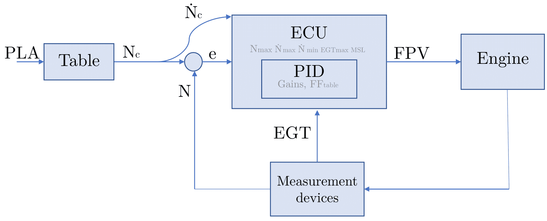
ECU Control aglorithm
Inputs
n_msd: Measured Speed from sensor. egt_msd: Exit Gas Temperature from sensor. pla: Power Level Angle demanded from pilot (value from sensor). fpv_resp: Fuel Pump Voltage to do respect. mode: Mode of execution:
 0 \(\Rightarrow\) Off: all variables set to zero. 1 \(\Rightarrow\) Checking: starter engine is commanded to max to check if engine is okay. 2 \(\Rightarrow\) Starting: pilot has total control with PLA once engine is runnning. V: Voltage to Engine.
Outputs
fpv: Fuel Pump Voltage to supply. tmp_prot: Boolean to active temperature protection. P: Proportional part of controller. I: Integral part of controller. D: Derivative part of controller. main_v: Voltage to main valve. ign_v: Voltage to Igniter valve. igniter: Voltage to igniter. starter: Voltage to starter engine.Configuration menu:

ECU Control block configuration
All parameters to be configured in the left column of the panel configuration constitute the engine characterization and must be filled in with the user’s engine specifications.
PID configuration: Users must configured the PID scheduler here. For more information on its configuration, check T-Sched PID section of this manual.
PLA / RPM: Users can enter the percentage of throtlle with respect to RPMs.
MSL / \(u_f\): Because atmospheric pressure decreases with altitude (MSL), a feed forward (\(u_f\)) is configured as a function of altitude in order to improve control at high MSL.
Fuzzy Logic Controller
The Fuzzy Logic Controller (FLC) block implements the Fuzzy Logic algorithm allowing users to perform robust control of any system.
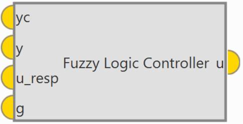
Fuzzy Logic Controller block
A FLC has to be embedded in a closed-loop control system.
Plant output is designed by \(u(t)\), its inputs are denoted by \(y(t)\), and reference input to the FLC is denoted by \(y_{c}(t)\). So, FLC will have \(y(t)\) and \(y_{c}(t)\) as controlled and commanded inputs, respectively, and \(u(t)\) as control output.
The FLC mathematical implementation in Veronte Autopilot 1x is the following:
The controller try to minimise the value of error, denoted by:
\[e_k = y_k - y_{ck}\]And it gets the value of change in error (derived from the error) \(ce(t)\) to do the fuzzy set:
\[ce_k = e_k - e_{k-1}\]Once is defined error and change in error, its values have to be pass to fuzzy values scaling it with its gains \(k_e\) and \(k_{ce}\) :
\[ \begin{align}\begin{aligned}en_k = k_e \cdot e_k\\cen_k = k_{ce} \cdot ce_k\end{aligned}\end{align} \]When these values are updated, the Membership Functions have to be defined as desired. Although their shapes could be any function (trapezoidal waveform, Gaussian waveform, etc.), they are usually triangular waveform.
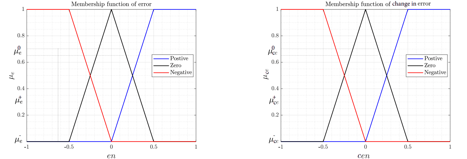
Example of membership functions of error and change in error
The exact values of the 2 last equations are used to get the weights \([\mu_{e}^{+} , \mu_{e}^{0} , \mu_{e}^{-}]\) and \([\mu_{ce}^{+} , \mu_{ce}^{0} , \mu_{ce}^{-}]\) . These values are obtained from error and change in error membership functions.
Then, those outputs must be arrange into a table, called the lookup table.
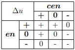
Example of Fuzzy Logic look up table
On the other hand, it is necessary to apply the fuzzy logic by this table, so it is checked the sign of \(en_k\) and \(cen_k\) , and the result is the membership function of the output to apply \(\Delta u\).
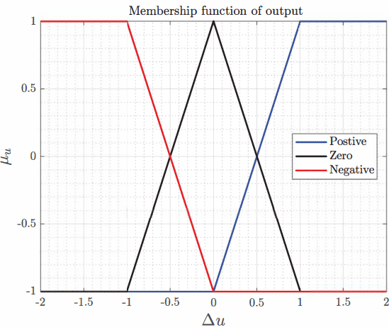
Example of membership function of output
Once the six values of weights \([\mu_{e}^{+} , \mu_{e}^{0} , \mu_{e}^{-}]\) and \([\mu_{ce}^{+} , \mu_{ce}^{0} , \mu_{ce}^{-}]\) are obtained, they must be combined in the nine possible combinations, selecting the minimum between both and getting its respective value of \(\Delta u\) in the output membership function.
The final value of output is obtained with the Center of Gravity method:
\[\Delta u = \frac{\sum_{i=1}^{9}\Delta u_{i} \cdot \mu_{i}}{\sum_{i=1}^{9} \mu _{i}}\]Finally, the real output value must be integrated in time and converted from fuzzy variables to real variables with its gain value \(k_u\) :
\[u_k = u_{k-1} + k_u \cdot \Delta u \cdot \Delta t\]
Inputs
yc: Desired set-point of the controlled variable. y: Value of the controlled variable. u_resp: Value of the output to do respect. g: Vector of controller gains.Output
u: Control output after controller.Configuration menu:
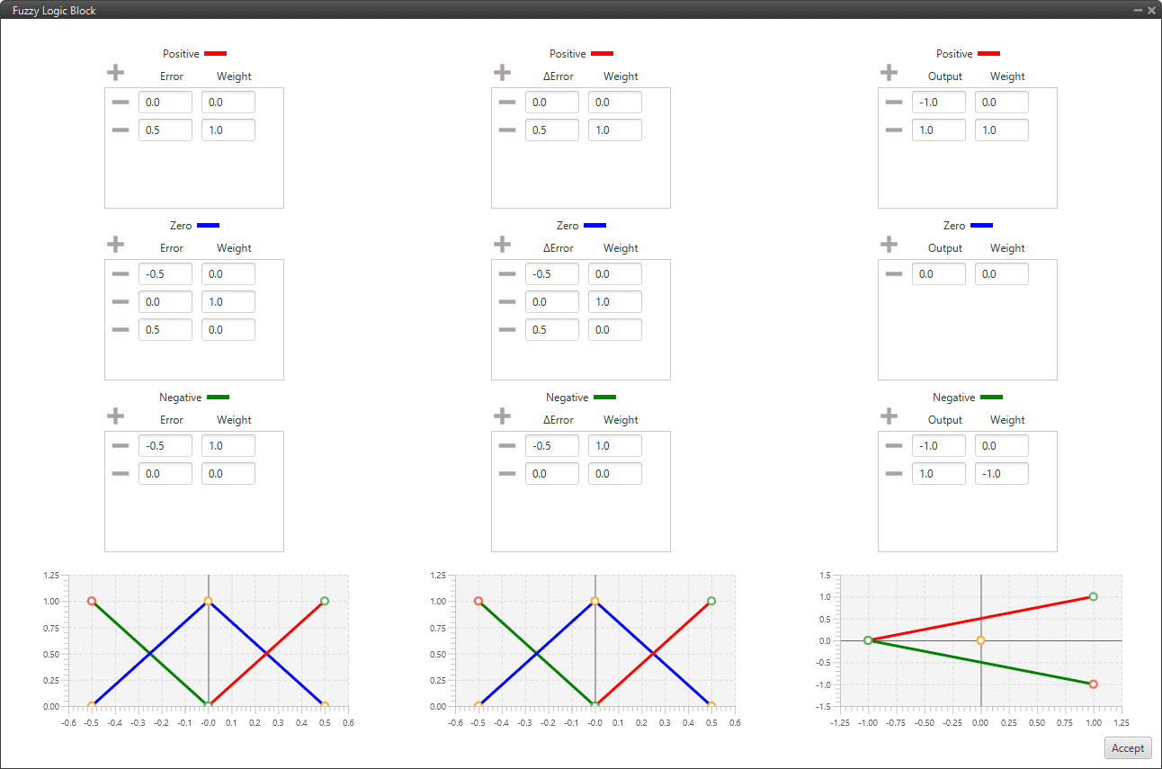
Fuzzy Logic Controller block configuration
These figures represent, respectively from left to right, the error membership function, the change in error membership function and the output membership function that have been explained above.
The user can configure these functions as desired by adding or deleting points.
Note
The default configuration is already designed for control.
Driver Control Filter
First, it is presented how the Adaptive-Predictive control algorithm has been implemented in blocks.
The part of the algorithm that tries to estimate the system transfer function (System Identification), the part that acts as a filter for the system output (Driver Control Filter) and the control part (Predictive control) are separated.
Therefore, Driver Control Filter block works together with the System Identification and the Predictive Control blocks for the Adaptative-Predictive control algorithm.
An example of use is shown below:
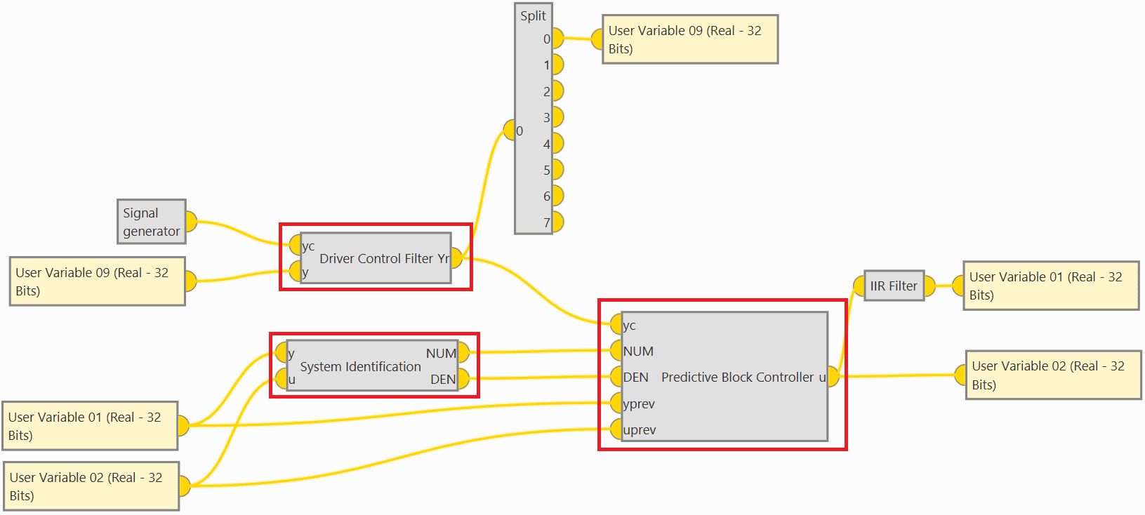
Adaptive-Predictive control blocks example
This example corresponds to the integration of a simulation. Therefore, an IIR Filter block and a Signal generator block have been added to simulate a real physical system, i.e. these blocks would not be needed in a real scenario:
IIR Filter simulates how the output responds to the input.
Signal generator simply simulates a desired input function.
Driver Control Filter block gives a vector with variables set points (SP) using a second order filter.
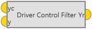
Driver Control Filter block
It acts as a 2-order filter with optimal coefficients for the Adaptive-Predictive control algorithm. These coefficients are calculated from the configurable parameters of the block.
Inputs
yc: Desired system output (Set Point). y: Measured system output.Output
Yr: Projected desired trajectory vector.Configuration menu:
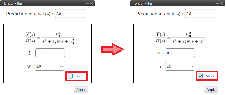
Driver Control Filter block configuration
The following parameters must be set:
Prediction interval (\(\lambda\)): Number of future instants (Prediction Horizon), how many samples are taken from the vector.
Shape: Depending on whether it is enabled or disabled, the paramters to be entered are different. Users can enable or disable it depending on the data available to them:
\(\zeta\): Damping ratio.
\(w_o\): Natural frequency.
Mp: Maximum overshoot.
Ts: Settling time (2% criteria).
Note
The relationships between the different parameters are:
\[Mp = \exp \left(-\zeta \cdot \frac{100 \cdot \pi}{\sqrt{1 - {\zeta}^2}} \right)\]\[Ts= \frac{4}{\zeta \cdot w_0}\]
System Identification
System Identification block gives the coefficients of the transfer function at Z-domain,
Where, \(A\) and \(B\) are polynomials in \(z\).

System Identification block
This blocks works together with the Driver Control Filter and the Predictive Control blocks for the Adaptative-Predictive control algorithm, as explained above.
Inputs
y: System output. This is the measurement. u: System input. This is the control action.Outputs
NUM: System coefficients numerator. DEN: System coefficients denominator.Configuration menu:
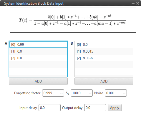
System Identification block configuration
Forgetting factor (\(\lambda\)): Determines how many inputs and outputs are taken into account for the estimation.
Recommended values between 0.98 and 0.995.
\(\delta_0\): Initial value of covariance matrix.
Noise (\(\gamma\)): From this noise threshold, the RLS (Recursive Line Square) is not calculated.
Input/Ouput delay: Given the input/output size, a delay is applied to the sample vector size.
Predictive Control Block
Predictive Block Controller gives the optimal control output given a dynamic model as a result of the system identification block.
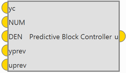
Predictive Control block
This blocks works together with the Driver Control Filter and the System Identification blocks for the Adaptative-Predictive control algorithm, as explained above.
Inputs
yc: Desired system output (SP) or trajectory. NUM: Numerator coefficients of system model plant. DEN: Denominator coeffcients of system model plant. yprev: Previous system output. uprev: Previous system input.Output
u: Control output.Configuration menu:
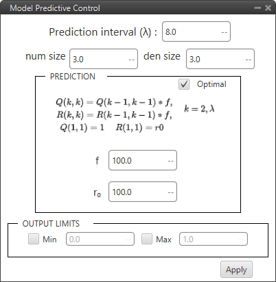
Predictive Control block configuration
The following parameters must be set:
Prediction interval (\(\lambda\)): Number of future instants (Prediction Horizon), how many samples are taken from the vector.
Optimal: Depending on whether it is activated or deactivated, the following parameters are auto-calculated or not.
f: If this factor is greater than 1, the past measurements have greater weight.
r₀ : If this factor is grater than 1, there is a more aggresive follow-up of the reference, on the contrary it is smoother.
Output Limits: Maximum and minimum limits for the controller output (for the control signal \(u\)).
Quaternion Control
Quaternion Control block for fixed multirotor aircraft.

Quaternion Control block
The Quaternion Control mathematical implementation in Veronte Autopilot 1x is the following:
The quaternion control algorithm calculates the desired direction and magnitude of the thrust vector of a multicopter in order to achieve the desired NED velocities, these generate a three-component acceleration vector in NED coordinates, which is compared with the actual direction of the thrust vector to obtain a quaternion representing the rotation from the actual to the desired thrust.
The error is applied to a control law determined by a time constant that provides the body angle rates to achieve the desired acceleration.
In addition, the algorithm is divided in two quaternion calculations depending on the yaw being controlled or not:
Reduced: Only the crucial angles of the thrust desired vector are considered. The yaw is not controlled directly.
Full: Both the pointing direction of the vector and the yaw is controlled.
Inputs
(Optional) attmode: Flag for velocity (hover) or angle (hold) control. If true only the angles will be controlled, if false or not connected the velocity of the aircraft will be controlled. (Optional) vnc: Desired north velocity (only used if velocity mode is active). Assumed zero if not connected. (Optional) vec: Desired east velocity (only used if velocity mode is active). Assumed zero if not connected. vdc: Desired down velocity. yawc: Desired yaw. (Optional) pitchc: Desired pitch (only used if angle mode is active). Assumed zero if not connected. (Optional) rollc: Desired roll (only used if angle mode is active). Assumed zero if not connected. (Optional) thr_sat: Saturated thrust from previous step. Used for respect and antiwindup.Outputs
rrc: Desired roll rate. prc: Desired pitch rate. yrc: Desired yaw rate. thr: Desired thrust.Configuration menu:
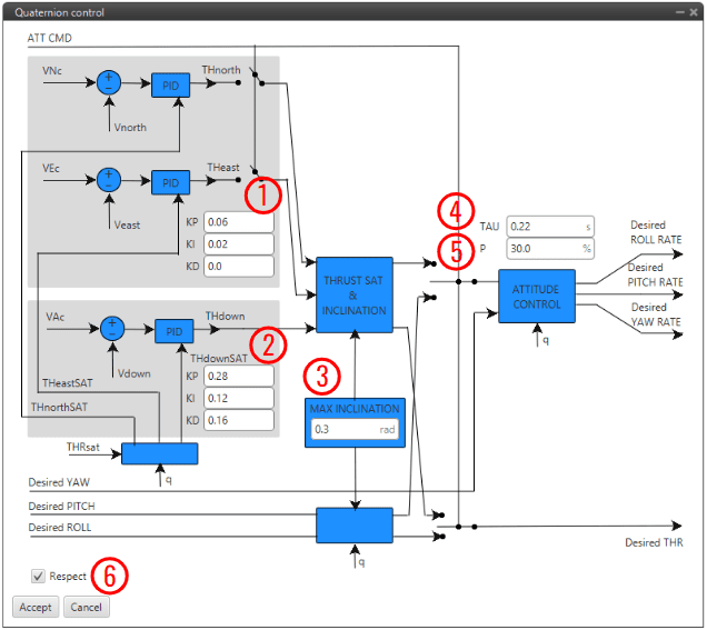
Quaternion Control block configuration
As this block is mainly constituted by 3 PID controllers (fore more infromation, see PID block), only some relevant parameters are detailed below:
PID to transform desired velocities into desired accelerations in NED.
PID to transform the vertical velocity into desired acceleration.
MAX INCLINATION: Maximum inclination allowed to the aircraft.
TAU: Time constant of the system. It is also the gain used for the feedback controller.
Recommended values between 0.1 and 0.25 seconds.
P: Reduction factor indicating how the yaw is to be controlled compared to pitch and roll.
The idea is that the “yaw control power” is lower in a multicopter as it is controlled by angular momentum difference between motors while pitch and roll is controlled by thrust difference.
By default, it is configured to 30%.
Respect: If enabled, when the block is executed for the firs time, an initial I value will be applied so that ‘thr’ = ‘thr_sat’ for the first iteration.
Furthermore, the thrust is assumed to be between 0 and 1. In case the user has other values for the thrust, it is recommended to use an Interpole block at the input and output to adjust the range between 0 and 1.
Total Energy Control
Total Energy Control block has been designed for the decoupling of the control of the speed and FPA in fixed-wing aircrafts. This block uses the internal navigation estimation.
It will provide two errors that must be minimized in order to obtain the desired speed and flight path:
Energy Distribution Error: Distribution of sistem energy between kinetical and geopotential energy. This error shall be used to control the aircraft’s pitch or FPA.
Energy Rate Error: Rate of change of the Total System Energy. This error accounts for the necessary increase or decrease in thrust.
The outputs Desired energy rate and Desired distribution energy rate are useful as feed forward in control.
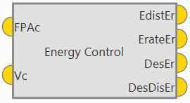
Energy Control block
Inputs
FPAc: Desired FPA (Flight Path Angle) set-point. Vc: Desired velocity set-point. Depending on the block configuration the velocity can be IAS or Ground Speed.Outputs
EdistEr: Energy distribution error for pitch control. ErateEr: Energy rate error for thrust control. DesEr: Desired energy rate. DesDisEr: Desired distribution energy rate.Configuration menu:
Some parameters of the Energy algorithm can be modified by double clicking on the block:
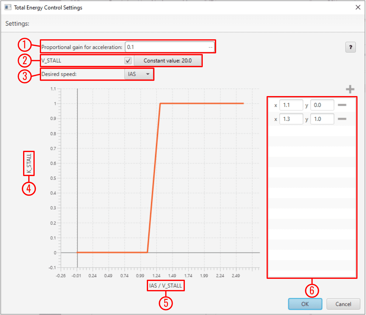
Energy Control block configuration
Proportional gain for acceleration: This is an indication of how aggresive the algorithm is when trying to gain speed. The higher the value, the faster the algorithm will try to ‘dive’ in order to gain speed.
A typical recommended value is around 0.1-0.3. Higher values are only recommended for fast maneuvering platforms.
V_STALL: Stall velocity parameter can be enabled or disabled. Users can manually enter this value or select a variable.
Desired speed: The user must choose between IAS and GS (Ground Speed) for reference. The use of GS is not recommended unless Airspeed measurement is not available.
K_STALL: Stall correction coefficient. If 1, energy control is balanced for altitude and speed. If 0 only speed control is taken into account.
IAS/V_STALL: Speed/Stall ratio. Ratio between current speed and minimum speed.
Stall correction interpolation function: Defines how the relationship between the stall correction coefficient and the Speed/Stall ratio works. The default configuration (as shown in the figure above) is recommended.
Note
The Stall correction coefficient is a Safety tool that can be used to sacrifice altitude control in order to improve speed control when speed gets close to the stall velocity (V_STALL) defined above.